10 Essential Steps for Single-Cell RNA-seq Analysis with Scanpy on PBMC Data

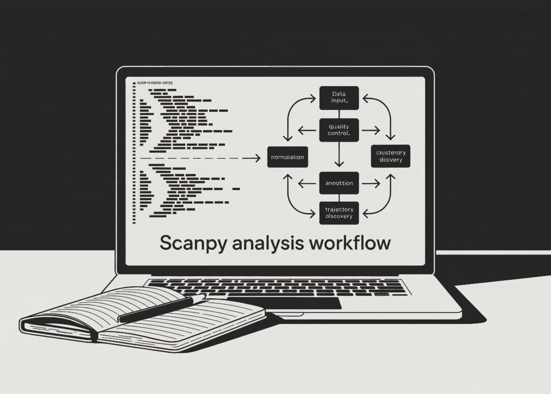
Single-cell RNA sequencing (scRNA-seq) has revolutionized our understanding of cellular heterogeneity. Analyzing the resulting high-dimensional data demands a robust pipeline. Scanpy, a scalable Python toolkit, offers a comprehensive workflow for preprocessing, clustering, annotation, and trajectory inference. In this guide, we walk through a 10-step analysis using the classic PBMC-3k benchmark dataset. Each step builds on the previous, from loading raw counts to saving a fully annotated AnnData object. Whether you are new to scRNA-seq or looking to refine your workflow, these steps provide a clear, reproducible path to extracting biological insights.

Step 1: Load and Inspect the PBMC Dataset

Begin by loading the PBMC-3k dataset, which contains 2,700 peripheral blood mononuclear cells. Using Scanpy's built-in dataset function, you obtain an AnnData object with raw counts in the X matrix and gene names in var_names. Make gene names unique to avoid duplicates. Inspect the object using print() to confirm dimensions and metadata. This initial exploration sets the stage for downstream quality control and analysis.

Step 2: Calculate Quality Control Metrics

Quality control (QC) is critical for removing low-quality cells and technical artifacts. Identify mitochondrial genes (starting with MT-) and ribosomal genes (RPS/RPL). Use Scanpy's pp.calculate_qc_metrics to compute per-cell metrics: number of genes detected, total UMI counts, and percentage of mitochondrial reads. Visualize these metrics with violin and scatter plots to spot outliers. High mitochondrial content often indicates dying cells, while very low gene counts may represent empty droplets.

Step 3: Filter Low-Quality Cells and Genes

Apply threshold-based filtering to retain only high-quality cells. Remove cells with fewer than 200 genes and genes detected in fewer than 3 cells. Further, filter out cells with more than 2,500 genes (potential doublets) and those with more than 5% mitochondrial reads. These thresholds are standard for PBMC data and eliminate debris, empty droplets, and damaged cells. The result is a clean dataset focused on viable, single cells.

Step 4: Detect and Remove Doublets with Scrublet

Doublets—two cells captured in the same droplet—can mask true biological variation. Use Scrublet to simulate doublets and score each cell's likelihood of being a doublet. After running sc.pp.scrublet, inspect the predicted doublet count and remove those cells. This step improves clustering accuracy and ensures that cell populations reflect real single cells, not artifacts.

Step 5: Normalize and Log-Transform Counts

Normalization accounts for differences in sequencing depth across cells. First, store raw counts in a layers["counts"] for later use. Then perform library-size normalization to a target sum of 10,000 per cell, followed by log transformation. This stabilizes variance and makes the data more amenable to statistical modeling. The log-transformed expression is the standard input for most downstream steps.

Step 6: Identify Highly Variable Genes

Focus the analysis on genes that vary the most across cells, typically those driving biological differences. Use Scanpy's pp.highly_variable_genes with default parameters (min_mean=0.0125, max_mean=3, min_disp=0.5) to select about 2,000 highly variable genes. Plot the selection to verify. Store the full dataset in adata.raw for later reference, then subset the object to only highly variable genes for efficient computation.

Step 7: Score Cell-Cycle Phases and Regress Unwanted Variation

Cell-cycle heterogeneity can confound clustering. Use Scanpy's cell-cycle scoring function (e.g., using known S and G2/M phase gene lists) to compute phase scores. Then regress out the effect of cell-cycle phase, total counts per cell, and mitochondrial percentage using linear regression. This step removes technical noise and biological variation that is not of primary interest, allowing clearer identification of cell types.

Step 8: Scale Data and Reduce Dimensionality

Scale the data to unit variance and zero mean, clipping extreme values to avoid undue influence. Then perform principal component analysis (PCA) to capture major sources of variation. Typically 50 PCs are sufficient. Visualize the PCA elbow plot to choose the number of components. Next, compute UMAP and t-SNE embeddings for visualization. These low-dimensional representations reveal cell neighborhoods and facilitate downstream clustering.

Step 9: Cluster Cells and Identify Marker Genes

Cluster cells using the Leiden algorithm on the neighborhood graph (built from PCA). This graph-based method is robust and scalable. After clustering, run differential expression tests (e.g., sc.tl.rank_genes_groups) to find marker genes for each cluster. Use canonical PBMC markers like CD3D for T cells, MS4A1 for B cells, LYZ for monocytes, etc., to annotate clusters with cell types. This annotation transforms clusters into biological interpretations.

Step 10: Explore Trajectories and Score Custom Signatures

For dynamic processes like differentiation, infer trajectories using PAGA (Partition-based Graph Abstraction) and diffusion pseudotime. These methods uncover lineage relationships and ordering. Additionally, compute a custom interferon-response score using a gene set of interest (e.g., IFIT1, ISG15). Finally, save the fully analyzed AnnData object to disk for future use. This comprehensive pipeline yields both static cell types and continuous transitions.

By following these 10 steps, you have built a complete single-cell RNA-seq analysis pipeline using Scanpy on PBMC data. From loading raw counts to trajectory inference, each phase is modular and can be adapted to other datasets. The resulting object contains clustering, annotations, and pseudotime, ready for downstream exploration or integration with other experiments. This workflow serves as a foundation for deeper biological discovery in diverse single-cell studies.